Lesson 3: Data formatting in excel!

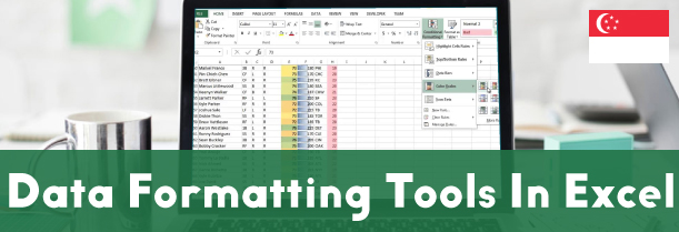
Data formatting tools in Microsoft excel!

This video is a part of free Excel Training Singapore, where I show you how to use Data formatting tools in Microsoft excel from the basics and also cover a lot of advanced Features.

Data formatting is a way of making any raw data look more presentable and readable by adding rows, columns, borders and colors to it. Data formatting allows you to fill in various cells with different color to differentiate between the important and non-important data. Data formatting gives the freedom to the user to format the painter that enables to add colors to the texts and calls as per the choice of the user.

Benefits of data formatting in excel –

• Data formatting in excel makes the data more polished and presentable by enabling you to add specific details to the cells.
• Data formatting makes data Understanding very easy because of its professional presentation.
• Data formatting in excel gives you the Choice to increase or decrease size of data or text stored in each cell.
• Data formatting enables one to perform various functions on data such as make the data bold, turn it to italics, underline the important data, add color to the border of the cell or double underline to highlight the data.
• Data formatting in excel allows one to Add colors to the text of the cell thereby beautifying the data and making it look more professional.
• Data formatting function allows user to change the color of the cell and the text written in it that helps to highlight the important data.
• Data formatting allows users to merge cells that increase the length and breadth of the Cell and store the entire text in one cell without breaking the cell in between.

How to access data formatting tools in excel? 

In Microsoft Excel there are many ways to access data formatting. To learn how to access data formatting, follow the steps mentioned below –

• In the home tab on the top left section of the excel, there are three options readily available which are font group, alignment category and the style category.
• Beginning with the font group, select any section of the raw data where you want to change the font.
• Click on the font group, a drop-down menu appears that contains all the available font options. As you move over the various fonts, the selected font keeps on changing.
• Click on which ever font you like the best and the entire selected raw data will appear in that font.
• In the alignment group you have the options to align your data at the top, middle or bottom by clicking on the align icon.
• Click on the orientation icon in the alignment group and choose the option of angel counter clockwise from the drop-down menu box.
• As soon as you click this option the text in the selected cell appears at an angle of 45 degrees and the row height of the cell gets adjusted accordingly.

How to use the cell styles? 

Cell styles enables you to fill the cell and it’s contents with a particular color that are pre decided by excel. You can customize the entire set as well. To perform these functions, follow the following steps –

• Click on cell styles option on the right side of the home tab.
• The drop menu appears and shows some of already pre populated sets.
• Select any of the set by right clicking on it and the cell’s color changes to that color.
• The text so typed in that cell will also appear in the color pre decided in that set.
• There are many other options in that same drop down such as heading 1, heading 2 and so on, each of them containing the details underneath it.
• You can customize your own set by clicking the option new cell style that open a new pop up box where you can easily edit the style of the box.

How to remove the remaining grids available on the work space!

While excel provides us with infinite count of rows and columns, in reality not all are used. To learn how to remove those cells and make your raw data appear cleaner, follow the following mentioned steps –

• Click on view option in the tool bar on the top most area of the screen.
• There appears an option “gridline” that has a box next to it.
• A tick on that box appears by default.
• Uncheck that box by simply clicking on that box. All the surplus or unused grid cells will be removed from the working area.

Learn Some Advanced Microsoft Excel Features in Singapore! 

Microsoft Excel Certification Course comes with certain features that gives the best utility when learned under the guidance of experts only. To gain such great command over Microsoft Excel join Skillsfuture excel Course in Singapore now!

This Tutorials covers the basics of data formatting in Excel.

You can change data according to their needs in Excel to make it look better and to highlight some data points. For example, if you have data-set and you want to highlight the negative numbers, you can simply highlight it in red color to it.

there are some of the common formatting features we use to make my data look better and more readable

• Applying borders to all cells
• Making headers bold
• Giving a background cell color to headers.
• Center align the headers
• You can find these options in Home tab in the Font category.

This video is a part of Excel Training Singapore where I show you how to use Excel from the basics and also cover a lot of advanced topics.